*Organ and Body Scale Team, Integrated Simulation of Living Matter Group, Computational Science Research Program, RIKEN, 2-1 Hirosawa, Wako-shi, Saitama, 351-0198, JAPAN **Oshima Laboratory, Institute of Industrial Science, The University of Tokyo, De505 4-6-1 Komaba, Meguro-ku, Tokyo, 153-8505, JAPAN ***Department of Mechanical Engineering, School of Engineering, The University of Tokyo, 7-3-1 Hongo, Bunkyo-ku, Tokyo 113-8656, JAPAN

Abstract

Traditional fluid-structure interaction techniques are based on arbitrary Lagrangian-Eulerian method, where strong coupling method is used to solve fundamental discretized equations. After discretization, resulting nonlinear systems are solved using an iterative method leading to set of linear subsystems. The resulting linear subsystem matrices are sparse non-symmetric indefinite with small or zero diagonal entries. The small pivots of these matrices may render the incomplete LU factorization unstable or inaccurate. To improve that, this paper proposes an approach that can be used together with a stabilization and offers an additional feature to be used to gain an advantage in its parallelization.

1. Introduction

The traditional fluid-structure interaction techniques (FSI) are based on the arbitrary Lagrangian-Eulerian method, where strong coupling method (direct method) is used to solve the fundamental discretized equations to satisfy the geometrical compatibility and the equilibrium conditions on the interface between the fluid and structure domains. The strongly coupled arbitrary Lagrangian-Eulerian method is used to address the added-mass effect, which is typical for loosely coupled time-stepping algorithms. After the discretization in space and time, the resulting nonlinear systems are solved using an iterative method, e.g. Newton-Raphson, leading to a set of linear subsystems that are then solved by linear sparse iterative solvers. The resulting linear subsystem matrices are sparse non-symmetric indefinite with small or zero diagonal entries. The small pivots of these indefinite matrices, associated with the small or zero diagonal entries, may render the incomplete LU factorization unstable or inaccurate. It is known that stabilization techniques, based on replacing the small diagonal entries with some large values on the matrix, can at least partially resolve the issue, however this paper proposes different approach that can be used together with the stabilization. Furthermore, the present technique of decomposing the system into smaller ones, offers an additional feature that can be used to gain an advantage in its parallelization to fully exploit the large scale parallel machines.

Preconditioned Krylov subspace methods are generally considered very suitable for solving very large sparse linear systems of the form

(1)

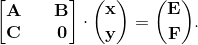
where K is an unstructured sparse stiffness matrix. However, when the matrix is indefinite, i.e. it has both positive and negative eigenvalues, the incomplete LU (ILU) preconditioning techniques can fail or become inaccurate. An indefinite matrix with zero diagonal entries may have higher chances of encountering zero pivots if the matrix is also non-symmetric [1,2], which is the typical case of the indefinite matrices arising from strongly coupled FSI applications.

Since small pivots are often the origin of the instability in computing the ILU factorization on an indefinite matrix, several works have been published on permuting large entries onto the diagonal of the indefinite matrix before solving the system [3-6].

In this paper, the system arising from an FSI application is decoupled into two subdomains, namely the fluid and structure subdomains. The stiffness matrix of each subdomain is formed separately, the two resulting systems are condensed by eliminating the interior nodal unknowns, the interface system is solved and the interior nodal unknowns are recovered at last. The areas of the global system with the zero diagonal entries are placed in the interface system, even though they do not necessarily belong to the interface. Thus, the systems for the interior nodal unknowns of the two subdomains no longer contain zero diagonal entries and are of good condition numbers.

2. Methods

In the present study, the applied FSI solver is a fully implicit, monolithic arbitrary Lagrangian-Eulerian finite element approach [7]. The discretization is based on the Q1/P0 finite element pair, where continuous piecewise linear approximation is used for the kinematic variables (displacement, velocity, acceleration) and discontinuous piecewise constant approximation for the pressure, together with Newmark-b scheme for time stepping. The resulting nonlinear systems are solved using a Newton-Raphson method, while the linear subsystems are treated via Krylov Subspace method, namely generalized minimal residual method with ILU preconditioner.

At each time step, the resulting linear subsystem is of the following form

(2)

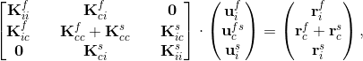
where the indexes s and f stand for the structure and fluid domains, respectively, u are the unknowns, r is the sum of the internal and external forces, the subscripts c and i denote the coupling parts and the internal parts of variables, respectively.

Let us consider the FSI analysis as a problem of two subdomains, namely the fluid and solid subdomains. The first step is to assemble the system matrix for each subdomain separately. Thus, instead of setting up the Eq. (2), two systems are assembled, one for each subdomain, as follows

(3)

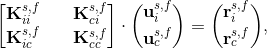
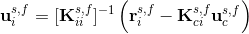
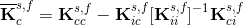
here, as before but in other words, subscript i stands for the internal degrees of freedom (DOFs) related to the nodes of the given subdomain except for the FSI-boundary nodes the DOFs of which are represented by the subscript c. Notice that the DOFs are organized in such a manner that all of those related to the FSI-boundary nodes are in the last rows and columns of the two systems. The system matrices can be, and in the case of the FSI linear subsystems are, non-symmetric, i.e. K_ci is not the transpose of K_ic.

In order to solve the FSI-boundary DOFs separately, condensation of the systems (3) is performed by deriving the u_i from the first equation of the systems as follows

(4)

and substituting it into the second equation of the systems. Thus, the resulting condensed systems are of the following form

(5)

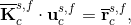
where

(6)

and

(7)

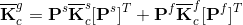
The condensed system matrix, , of each subdomain is then assembled to form a global matrix for the DOFs along the FSI boundary as follows

(8)

and similarly with the right hand side

(9)

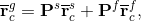
where g denotes the global system of the FSI-boundary related unknowns and the matrix P represents the permutation matrix for converting the DOFs of the given subdomain to the global system, which is of following form

(10)

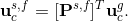
Solving the system of Eq. (10) gives the solutions for the DOFs along the FSI boundary, i.e. u_c^g.

Consequently, the internal DOFs for each subdomain are recovered using the Eq. (4); but first, the global boundary unknowns have to be converted back to the local systems by

(11)

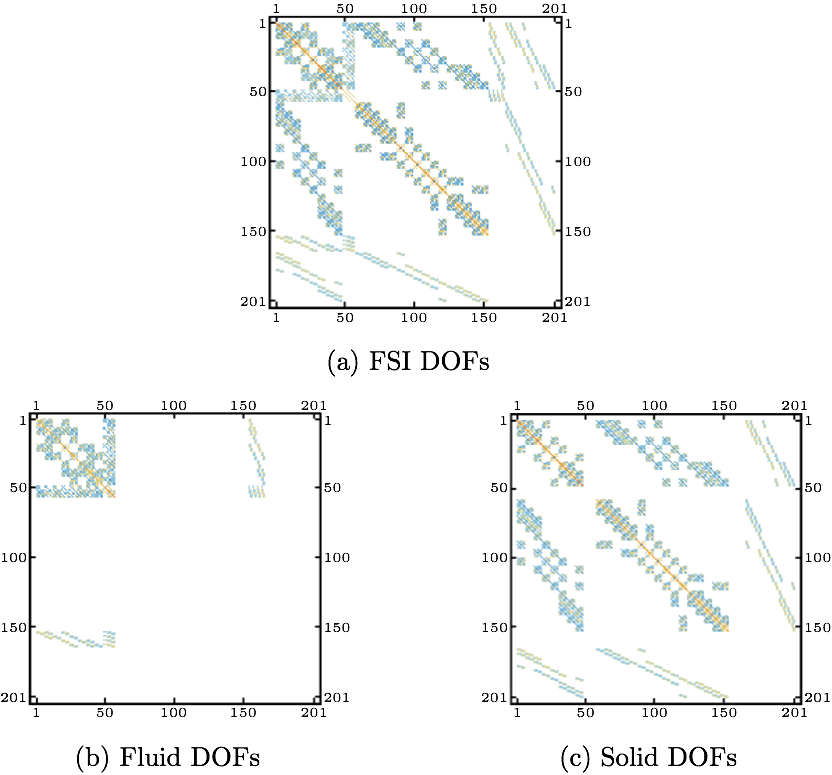
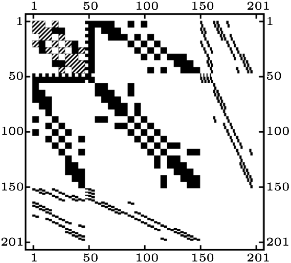
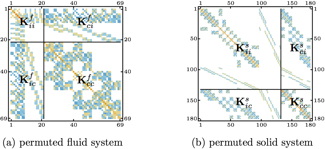
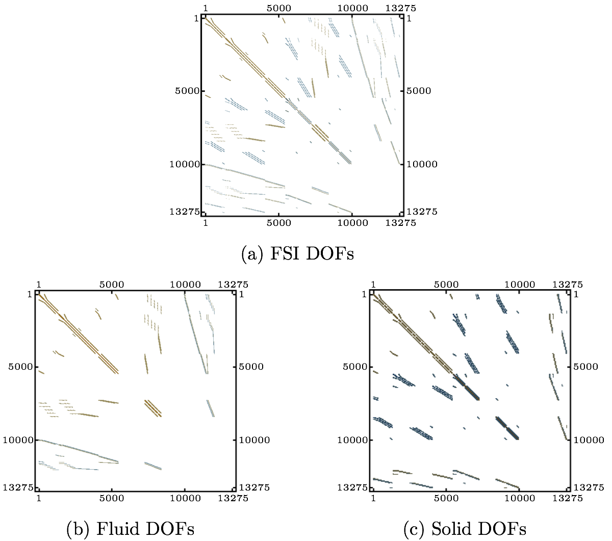
Now, the interior nodal unknowns can be solved according to the Eq. (4).

Fig. 1(a) shows an example of a system arising from strongly coupled FSI application based on the Q1/P0 finite element pair discretization. The white areas are those with zero or very small entries. Fig. 1(b) and (c) depict the DOFs related to the fluid and structure domains of the FSI system, respectively. Needless to say, the parts common for both Fig. 1(b) and (c) are those related to the FSI boundary, as shown in Fig. 2, distinguished by the striped area.

Figure 1: The sparsity of an FSI system, Eq. (2) (201 DOFs), (a) and its decomposition into fluid (b) and solid (c) DOFs before reordering.

Figure 2: Identification of the FSI-boundary DOFs (striped).

An important way of quantifying the accuracy of the solution of a linear system is by computing the condition number κ(K), defined as follows for a suitable choice of the norm

(12)

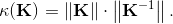
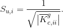
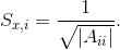
If the condition number of a matrix is large, the matrix is said to be ill-conditioned. If κ(K)=10^k the loss of at least k digits of precision in solving the system (1) can be expected [8]. The matrix shown in Fig. 1(a) has the condition number κ(K)(=||K||_∞·||K^-1||_∞)=2.4·10¹⁹. Therefore, solving such a system requires a preconditioning, usually ILU with high level fill, which as mentioned above can fail or become inaccurate when dealing with indefinite matrices.

The matrix is of small dimensions for a matrix arising from an FSI application. To simplify the explanation of the method, a very simple FSI example is used in this section. The number of DOFs is 201. The matrix has both positive and negative eigenvalues, thus is considered indefinite.

To create the systems (3) for the solid and fluid subdomains, the matrices from Fig. 1(b) and (c) have to be reordered in the manner mentioned above, i.e. all of the DOFs related to the FSI boundary are to be placed in the last rows and columns of the systems. First, the zero rows and columns have to be removed, as shown in Fig. 3.

Figure 3: The fluid (a) and solid (b) systems after removal of the zero rows and columns.

Now, the number of the DOFs of the fluid and solid systems are 69 and 180, respectively. Out of those, 48 fall under the FSI-boundary DOFs, i.e. those shared by both domains. As mentioned above, the discretization is based on the Q1/P0 finite element pair, where continuous piecewise linear approximation is used for the kinematic variables and discontinuous piecewise constant approximation for the pressure. Thus, the kinematic variables are covered by the first 57 and 144 DOFs of the fluid and solid systems, respectively. The DOFs representing the approximation of the pressure variable are covered by the rest of the systems, distinguishable by the zero (or very small) diagonal entries.

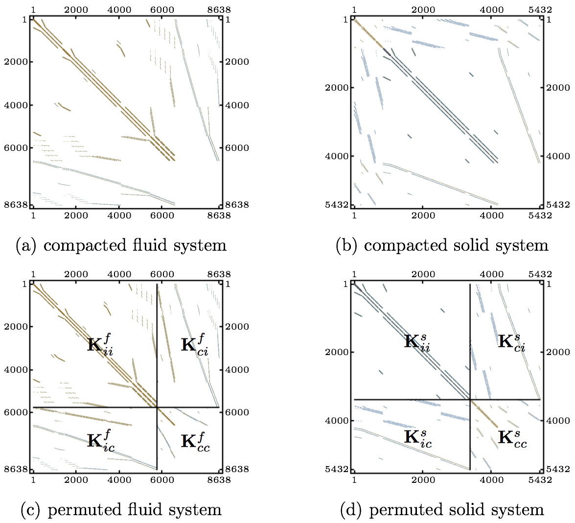
Fig. 4 shows the two systems after the rows and columns have been permuted in order to place the FSI-boundary related DOFs in the last rows and columns of the systems to reach the configuration of Eq. (3). The association with the system matrix of Eq. (3) is expressed in Fig. 4 using the notation from the equation.

Figure 4: The fluid (a) and solid (b) systems after permuting the FSI-boundary DOFs.

According to Eqs. (6) and (7), the inverse of the K^s,f_ii parts of the system matrices of the two domains is supposed to be found. However, the zero diagonal entries are now entirely carried by these parts of the system matrices. The resulting condition numbers are κ(K^f_ii)=4.7·10²⁰ and κ(K^s_ii)=1.2·10¹⁹. Since the result for inverse of badly conditioned matrix may contain significant numerical errors, this approach does not provide any advantage.

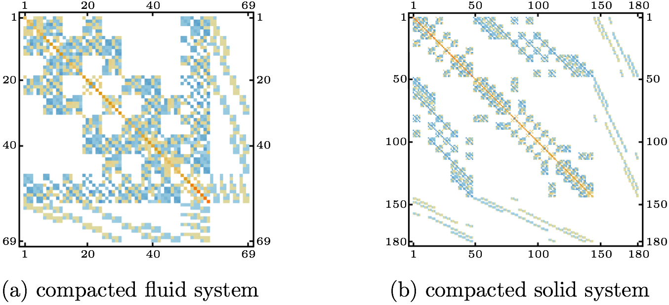
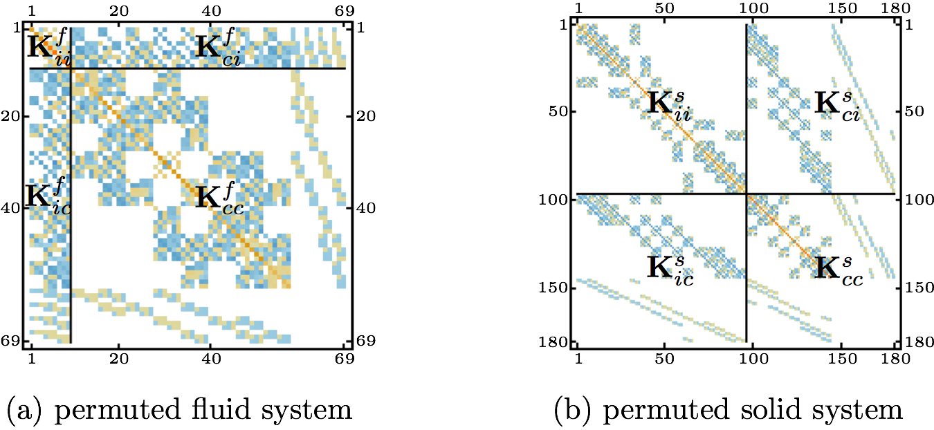
It is more convenient to move the DOFs coming from the P0 approximation to the K^s,f_cc parts of the system matrices, as shown in Fig. 5. From the physical point of view, those DOFs do not belong to the FSI boundary, but it is more convenient to carry them in the K^s,f_cc, where it becomes an issue when solving Eq. (10), rather than attempting to find the inverse of a badly conditioned matrix. The condition numbers κ(K^s,f_ii) now become 18.4 and 3.4, respectively.

Figure 5: The fluid (a) and solid (b) systems after permuting the FSI-boundary DOFs together with the P0 related DOFs.

The inverse operation in Eqs. (6) and (7) is computed by LU decomposing the well conditioned K^s,f_ii and then backsubstituting with the columns of K^s,f_ci and the vector r^s,f_i, respectively.

The global matrix for the DOFs along the FSI boundary, Eq. (8), is assembled combining the matrices from Eq. (6). The resulting pattern of the matrix is shown in Fig. 6(a). Depending on the origin of the appropriate DOFs, the matrix has different orders of magnitude. The area with the order of 10^-3 corresponds to the kinematic variables. The rest is the DOFs corresponding to the pressure variable either from fluid (-11,-12) or solid (-13,-21) elements, see Fig. 6(a).

Figure 6: The global matrix for the DOFs along the FSI boundary and the respective average orders of magnitude.

The matrix has no longer zeros on the diagonal. The order of 10^-21 is too small for a well conditioned matrix though. The condition number of the matrix is 1.47·10¹⁹. However, now that there are no zero members on the diagonal, it is rather straightforward to scale the system to improve its condition number. The system (1) is scaled using a scaling strategy ensuring unit diagonal entries, as explained in Appendix A.

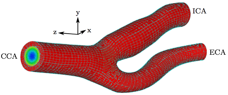
Using the full Gauss condensation to solve the un-decomposed FSI system, the accuracy of the solution is 1.4·10^-8, while solving it without the scaling, Eq. (A.9), is impossible. As mentioned above, the small pivots of these indefinite matrices, associated with the small or zero diagonal entries, may render the incomplete LU factorization unstable or inaccurate. The minimum pivots of the systems in Eq. (2), Eq. (2) with scaling as in Eqs. (A.9), and (10) with scaling as in Eq. (A.2), are 8.7·10^-20, 5.2·10^-6 and 1.8·10^-6, respectively.

However, Gauss condensation is a direct method; preconditioned Krylov subspace methods, e.g. generalized minimal residual method (GMRES), are generally considered suitable for solving these kinds of systems. When GMRES with diagonal ILU preconditioner is used to solve the original un-decomposed system in Eq. (2), the convergence is reached in 40 iterations with the tolerance of the method set to 10^-12. With the method presented here, i.e. solving the system decomposed in more steps, the convergence is reached in 7 iterations when solving Eqs. (10) and (4) is solved directly backsubstituting with a vector. The accuracies of the final solutions, ||K·u-r||₂, are 1.9·10^-18 and 5.3·10^-21 for the un-decomposed and decomposed systems, respectively. It is worth to note here, that GMRES method computes a sequence of orthogonal vectors, and combines these through a least-squares solve and update. It requires storing the whole sequence, so that a large amount of storage is needed. For this reason, restarted versions of this method have to sometimes be used. In restarted versions, computation and storage costs are limited by specifying a fixed number of vectors to be generated. This method is useful for general nonsymmetric matrices. For the here presented example, this was not an issue and the restarted version of this method was not used.

3. Results

A very simplified FSI example is used in the above section to explain the method. In the following, when presenting the actual FSI application, larger problem set of 13,275 DOFs is used. The model representing subject-specific common carotid artery is shown in Fig. 7, where the upper layers in red represent the blood vessel, i.e. the structural part of the FSI. The common carotid artery bifurcates into an internal carotid artery (ICA) and an external carotid artery (ECA). In the actual application, at the inlet (CCA), pulsatile flow is prescribed varying in time according to the measured data profile and the outlets (ICA and ECA) of the model are connected to the inlet of a 1D model providing non-zero pressure values based on the resulting flow rates at the outlets (see [7] for more details).

Figure 7: Model of the actual FSI example used.

The sparsity patterns of the FSI, fluid and structure domain systems are shown in Fig. 8, respectively.

Figure 8: The sparsity of an FSI system (13275 DOFs) (a) and its decomposition into fluid (b) and solid (c) DOFs before reordering.

3.1. Condition number

The condition number of the FSI system shown in Fig. 8(a) is 2.7·10¹⁹. The condition numbers of the Kii matrices for the solid and fluid domains without the P0 related DOFs, as depicted in Fig. 9(c) and (d), are 196 and 71, respectively. Thus, the products including the inverse of the Kii matrices in Eqs. (4), (6) and (7) can be solved using direct solvers without the need for preconditioning. Similarly as with the smaller example above, the accuracy of 10 9 is reached with 285 iterations within the GMRES algorithm when solving the un-decomposed system in Eq. (2). Whereas when solving the system decomposed into two subdomains and the shared DOFs, i.e. solving the smaller system in Eqs. (10) and (4) being solved using a direct method, respectively, the same accuracy is reached in 12 iterations.

Figure 9: The fluid (a) and solid (b) systems after removal of the zero rows and columns and fluid (c) and solid (d) systems after permuting the FSI-boundary DOFs together with the P0 related DOFs.

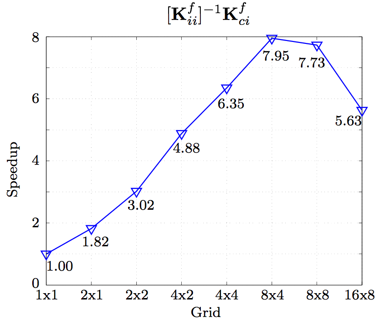
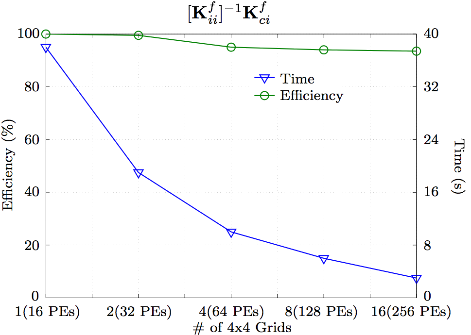
3.2. Performance

It is always a question of precision and performance, less performance for the price of more precision and vice versa. The GMRES method used to solve the un-decomposed original system, Eq. (2), needs more iterations and can not reach a precision that can be reached when solving Eq. (10). On the other hand, dividing the system into more smaller and better conditioned ones requires more operations to compute. The K_ii matrix is now well conditioned, but computing the products involving it requires time that can not compete with the time when the system is solved directly without it being divided into smaller parts. Time-wise, compared on single process, the operations required, when decomposing the full FSI system, take around four times more than the GMRES iterative method. However, it provides more room for parallelization.

4. Parallelization

If precision is not the issue, the system, being solved sequentially, is better off without the decomposition as proposed in this paper. However, the direct methods dealing with the well conditioned K_ii matrix are parallelizable with good scalability, which is an issue when using iterative methods, especially with preconditioning, which is the case most of the times in FSI applications. In parallel computation, the processor with maximum execution time governs the overall execution time, plus careful balance between the amount of computation and communication has to be reached, especially on large scale parallel machines. The exact way to parallelize the LU decomposition is not trivial, so this is discussed elsewhere. However, LU decomposition allows some clever parallelization, that is already exploited by solvers like SuperLU [9-11], PARDISO [12,13] and MUMPS [14-16].

In this paper, the SuperLU solver is used everywhere possible when decomposing the FSI system using Eqs. (4)-(11). For example, when treating Eq. (6), K^-1_iiK_ci is solved using the SuperLU solver, i.e. the K_ii is the system matrix entering the solver and the K_ci are the right hand sides.

The solvers, however, may not provide good efficiency for very high number of processors (PEs). The graph in Fig. 10 shows the speedup of the fluid K_ii as the system matrix, being solved with the fluid K_ci as the right hand sides of the system. The number of rows and columns of the system matrix is 5775 and the number of the columns of the K_ci matrix, in this case number of the right hand sides of the system, is 2508. The grid represents number of rows to number of columns by which the system matrix is divided when being factorized.

Figure 10: The speedup of the solution of the system with the system matrix being solved on different grids.

The aim of this study is to push the parallelization even farther, using the advantage provided by the decomposition of the FSI system. Now, the number of right hand sides, i.e. number of the columns of matrix K_ci, is also relatively large. This can be used for the farther parallelization by splitting the columns of the K_ci onto more PEs. This is briefly described in the following 6 points.

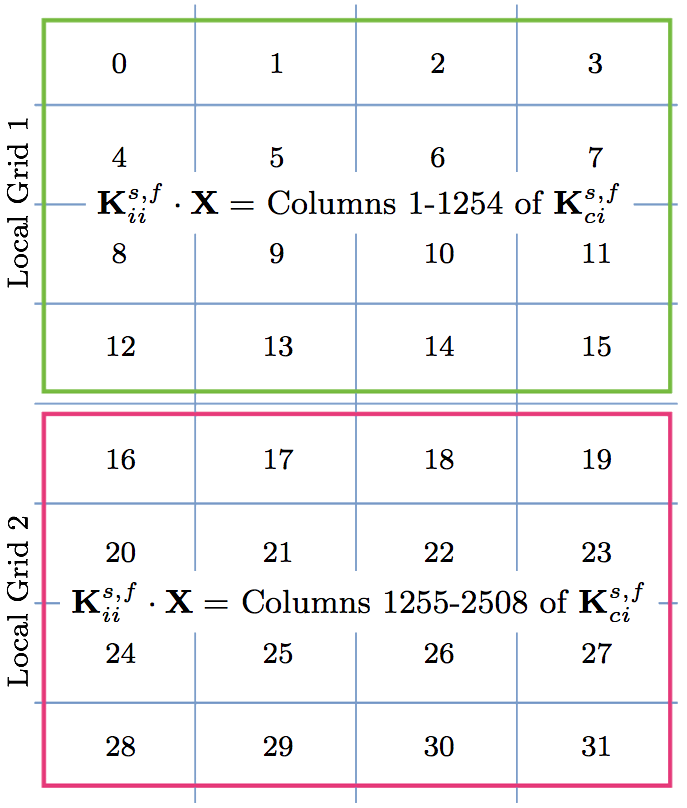
 (1) Initialize the MPI environment global SuperLU process grid.
 (2) Permute the rows and columns as depicted in Fig. 5.
 (3) Isolate the K_ii matrix and broadcast it to all PEs on the global grid.
 (4) Initialize N local SuperLU process grids, where N·(localgridsize)=globalgridsize.
 (5) Isolate the appropriate columns of the K_ci matrix for each of the local grids and broadcast it to all the PEs on the given local grid.
 (6) If there are N local grids, call SuperLU solver to solve the K^-1_iiKⁿ_ci, where n = 0, 1, ..., N. In other words, the Kⁿ_ci are the right hand sides different for each local grid.

Fig. 11 shows an example of how the K_ci matrix is split onto two local grids, i.e., for the fluid domain, the total number of the 2508 columns of the K_ci matrix is split between the two local grids. In other words, K_ii is factorized on a local grid of 4×4 twice, once on cores 0-15 with the first 1254 columns of the K_ci matrix and then second time (in parallel with the first local grid) on cores 16-31 with the second half of the K_ci columns.

Figure 11: An example of splitting the right hand sides onto two local grids.

Fig. 12 represents the outcome of the procedure summarized in the 6 points described above. The factorization of the system matrix is always performed on 4×4 local grid and the K_ci matrix, i.e. the right hand sides, is split using several of these grids. Thus, as stated above in the point (4), e.g. when using N = 16 of the local grids, 16·(4×4) = 256 PEs are used in total.

Figure 12: The times and the efficiency of splitting the right hand sides onto different number of 4×4 local grids.

Eq. (6) is then computed further by multiplying the K_ic with the result of the SuperLU solver on the K^-1_ii, i.e. K_icK^-1_iiKⁿ_ci. Again, this is performed using efficient parallel algorithm for matrix-matrix multiplication [17,18], on the local grids in parallel with no communication between them. The same applies to the subtraction of the appropriate columns of the matrix Kⁿ_cc and the result of the K_icK^-1_iiKⁿ_ci operation. Thus, the algorithm for the parallelization of Eqs. (4)-(11) continues as follows:

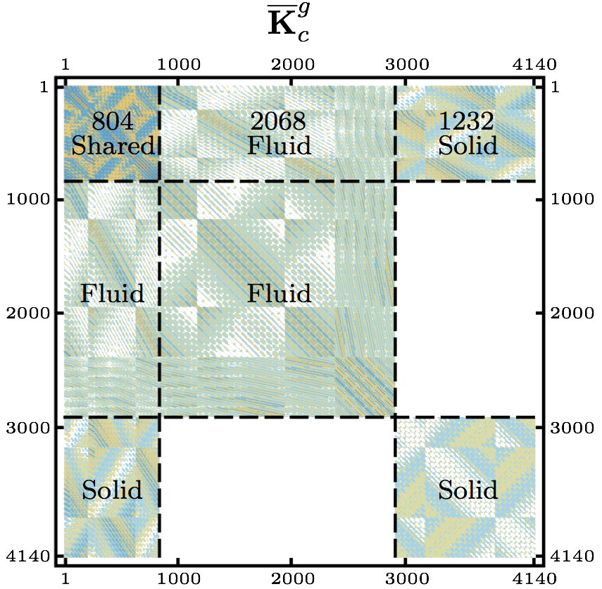
 (7) Isolate the K_ic matrix and broadcast it to all PEs on the global grid.
 (8) Isolate the appropriate columns of the K_cc matrix for each of the local grids and broadcast it to all the PEs on the given local grid.
 (8) Call the function DGEMM (calculates the product of double precision matrices) for matrix-matrix operation C=αAB+βC, where α and β are scalars, in this case -1 and +1, respectively and A, B and C are matrices, where A represents the K_ic matrix, B is the output of the SuperLU solver computing the K^-1_iiKⁿ_ci, and C is the Kⁿ_cc matrix.

Eq. (7), computing the condensed right hand side , is treated the same way and is included in the computation of Eq. (6). In other words, the r_i vector becomes part of the K_ci as the last column of the matrix. Equally, the r_c vector becomes part of the K_cc as the last column of the matrix. Thus, the resulting will be the last of column of the matrix on the last local grid, when the points (1)-(9) are being executed. This is not included in the above description of the points of the algorithm in order to keep it less complicated.

To assemble the global matrix, , for the shared DOFs along the FSI boundary, Eq. (8), the resulting matrices, and , are to be used. Thus, for the first time in the algorithm, the local grids need to communicate in order to exchange the necessary information. At this point, each of the local grids keeps part of the and matrices. To continue the following points of the algorithm, it is necessary to mention, that the system matrix entering the SuperLU solver is in compressed row storage format, i.e. the values of the nonzero elements of the matrix, as they are traversed in a row-wise fashion, are stored in one (double precision) vector, the column indexes of the nonzero elements are stored in second (integer) vector and the locations in the second vector that start a row are stored in third (integer) vector.

 (10) Send the resulting matrix from point (9) from the first PE of each local grid to the PE 0 of the global grid.
 (11) Receive it on PE 0 of the global grid from the first PE of each local grid.

The first PE of the first local grid is the PE 0 of the global grid, thus no communication (sending/receiving) is needed regarding the first local grid; and the communication between the other local grids and the PE 0 of the global grid are only between the first PE of each local grid and PE 0 of the global grid. Therefore, if there are N local grids, only N 1 PEs are sending the necessary information to the PE 0 of the global grid. The and vectors are extracted from the last column of resulting matrices of the last local grid.

The rest of the algorithm is rather straightforward.

 (12) Upon receiving the and partial matrices from the first PE of each (except for the first one) of the local grids, assemble the in compressed row storage format on PE 0 of the global grid.
 (13) Assemble the .
 (14) Call the SuperLU solver on given grid of user's choice with the as the system matrix and as the right hand side (one column).

At the point (14), the u^g_c is returned. The SuperLU is working on a given grid of a users choice. Generally, at this point, Eq. (10) can be solved efficiently on a grid of higher dimensions. Due to the operations in Eq. (6), the is not sparse matrix. As can be also seen in Fig. 13, the number of nonzero elements of the matrix is equal to (DOFs^shared + DOFs^fluidP0 + DOFs^solidP0)² - 2·DOFs^fluidP0·DOFs^solidP0, which in case of the example in Fig. 13 is (840 + 2068 + 1232)² - 2·2068·1232 = 12,044,048 nonzero elements. If there were no zero elements in the matrix, the number would be (DOFs^shared + DOFs^fluidP0 + DOFs^solidP0)² = 17,139,600, which means that around 70% of the matrix are nonzero elements. This number does not yet exceed the memory capacity of usual computer architecture, but many larger FSI models computed this way would have reached the limit. That could be the bottleneck of this method. However, the SuperLU offers the possibility of distributed input interface, i.e. the input matrices are distributed among all the processes. The distribution is based on block rows. That is, each process owns a block of consecutive rows of the matrices. If there is sufficient memory, the interface, where the input matrices are globally available (replicated) on all the PEs, is faster than the distributed input interface, because the latter requires more data redistribution at different stages of the factorization algorithm. All other matrices, namely K_ic, K_ii, K_ci and K_cc, are of high sparsity and do not need to be distributed in blocks.

Figure 13: The global matrix for the shared and P0-related DOFs along the FSI boundary.

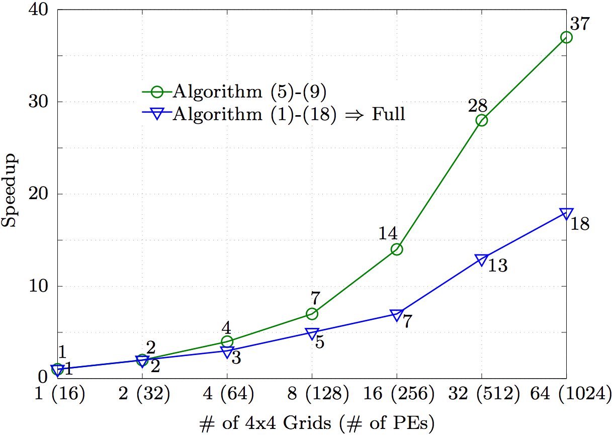
The matrix consists of the matrices and , as shown in Fig. 13, which are now split column-wise per each local grid. Each local grid carries specific number of columns of the two matrices and given rows of these column groups have to be sent to the appropriate PE to create the distributed input interface which is based on block rows. Thus, in case of the distributed input, the points (10)-(12) of the algorithm are as follows:

 (10) Send given block of rows of and from each local grid to the appropriate PE.
 (11) On given PE, receive the appropriate block of rows from each local grid.
 (12) Upon receiving the given block of rows of and from each local grid, assemble the block of rows of for the current PE.

Either way, the u^g_c is returned and the algorithm to parallelize the Eqs. (4)-(11) continues.

 (15) Set the global boundary unknowns back to the local systems for the fluid and solid domains, Eq. (11).
 (16) Isolate the K_ci matrix and broadcast it to all PEs on the global grid.
 (17) Compute the r_i-K_ciu_c using the DGEMV for matrix-vector operation.
 (18) Call the SuperLU solver on given grid of user's choice with the K_ii as the system matrix and result of the matrix-vector multiplication from the previous point as the right hand side (one column).

The last point of the algorithm computes Eq. (4) to recover the internal DOFs for both the fluid and solid domains.

Fig. 14 shows the resulting speedup of solving Eqs. (4)-(11) after the algorithm is applied. The factorization of the system matrices K^sf_ii is set to different numbers local grids of 4×4 size. If 64 groups of 4×4 local grids are used, then 64·(4×4) = 1024 PEs are used in total. The circular data symbols in Fig. 14, representing the speedup of solving the system [K^f_ii]^-1K^f_ci, can be compared with the results in Fig. 10 when the right hand side matrix K^f_ci is not being split among different groups of PEs.

Figure 14: Speedup of the computation within the entire algorithm, (1)-(18), and of the points from (5) to (9) where the columns of the right hand side matrix Kfci are being split among more local grids of 4×4 size.

5. Conclusion

Smaller well conditioned systems are being solved instead of one badly conditioned one. It would be possible to decompose the system to two parts only, where the coupled DOFs are carried within one of the systems, but then the advantage of having one system responsible for carrying the P0-related DOFs would be lost. This way, when K_ii does not carry the DOFs with zero diagonal entries, the condensed system global matrix Kcg, carrying these DOFs, also becomes free of the zero diagonal entries. Thus, this method serves as a conditioner too by filling the zero diagonal entries through the matrix operations in Eq. (6). Performance wise, if the precision is not the issue and only sequential way of computing is available at the moment, it is better to solve the system using solvers specially suitable for these kinds of system matrices. However, when the need for parallelization arises, indirect iterative solvers with preconditioning do not give much room for parallelism as there is too much dependency on the previous steps. Thus, having the option to use solvers with high level of scalable computing is a necessary part of the programming techniques required to exploit the speed of the parallel architecture of supercomputers. However, the room for parallelization of the solvers is limited in some extend either way. In order to push the parallelization even further, the [K^sf_ii]^-1K^sf_ci system, having the K_ci matrix as right hand side with large number of columns, is used to gain additional room for parallelization. The results show significant improvement in the scalability compared to when limiting the parallelization to the factorization of the system matrices only.

Acknowledgments

This research is supported by the Research and Development of the Next-Generation Integrated Simulation of Living Matter, as a part of the Development and Use of the Next-Generation Supercomputer Project of the Ministry of Education, Culture, Sports, Science and Technology (MEXT), Japan. Numerical calculations were conducted on the RIKEN Integrated Cluster of Clusters (RICC), more precisely the Massively Parallel Cluster (8192 cores). Also, thanks goes to Thomas M.H. Pham for proofreading in English.

Appendix A

Letting

(A.1)

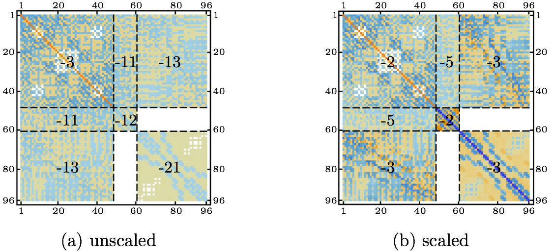
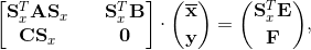
the solving system is scaled into following form

(A.2)

where the scaling factors are chosen as follows

(A.3)

Thus, the resulting block matrix has unit diagonal entries. The scaling yields a system with smaller range of the orders of magnitude as shown in Fig. 6(b). The condition number of such matrix is now 5.7·10⁷, i.e. of 12 orders less than before scaling.

After obtaining the solution of Eq. (10) and applying the permutation matrix in Eq. (11), the internal DOFs are recovered using Eq. (4), where the LU decomposition of the well conditioned K^sf_ii matrix has already been found before when computing Eqs. (6) and (7) and thus only the backsubstitution with the product of r^sf_i-K^sf_ciu^sf_c is necessary.

When Eq. (10) is solved using the full Gauss condensation, the accuracy of the global solution, consisting of the solutions u^fs_c and u^sf_i, computed as ||K·u-r||₂ is 1.3·10^-8. To compare, the full system matrix, from Eq. (2), is also scaled in a similar manner. However, the original system has zero diagonal entries, thus requires off-diagonal scaling. The global system has the following form

(A.4)

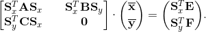
Now two diagonal scaling matrices are used, S_x and S_y. Letting

(A.5)

the system is scaled into form

(A.6)

where, as before, the scaling factors are chosen as

(A.7)

Scaling of variable y is enforced next via

(A.8)

to yield

(A.9)

By choosing S_yi to be the inverse of the largest element in column i of the block matrix S^T_xB, the coefficients in each column of the resulting block matrix S^T_xBS_y are no longer larger than unity. Since entries of the matrix C are of the same orders of magnitude as in the matrix B, the coefficients in each column of the resulting block matrix S^T_yCS_x are, in general, also no longer larger than unity. Thus, the scaled system has unit diagonal entries for matrix A and entries in matrices B and C smaller than unity.

REFERENCES

[1] Saad Y. ILUT: a dual threshold incomplete LU factorization. Numer Linear Algebra Appl 1994;14:387-402.
[2] Zhang J. A multilevel dual reordering strategy for robust incomplete LU factorization of indefinite matrices. SIAM J Matrix Anal Appl 2000;22 (3):925-47.
[3] Benzi M, Haws J, Tuma M. Preconditioning highly indefinite and non-symmetric matrices. SIAM J Sci Comput 2000;22:1333-53.
[4] Duff I. Algorithm 575: permutations for zero-free diagonal. ACM Trans Math Softw 1981;7:387-90.
[5] Duff I, Koster J. The design and use of algorithms for permuting large entries to the diagonal of sparse matrices. SIAM J Matrix Anal Appl 1999;20:889-901.
[6] Duff I, Koster J. On algorithms for permuting large entries to the diagonal of a sparse matrix. SIAM J Matrix Anal Appl 2001;22:973-96.
[7] Toma M, Krdey A, Takagi S, Oshima M. Strongly coupled fluid-structure interaction cardiovascular analysis with the effect of peripheral network. J Inst Ind Sci, The University of Tokyo 2011;63(3):339-44.
[8] Cheney W, Kincaid D. Numerical mathematics and computing. 6th ed. Publisher Brooks Cole; 2007.
[9] Demmel J, Gilbert J, Li X. An asynchronous parallel supernodal algorithm for sparse Gaussian elimination. SIAM J Matrix Anal Appl 1997;20(4):915-52.
[10] Demmel J, Eisenstat S, Gilbert J, Li X, Liu J. A supernodal approach to sparse partial pivoting. SIAM J Matrix Anal Appl 1999;20(3):720-55.
[11] Li X, Demmel J. SuperLU-DIST: a scalable distributed-memory sparse direct solver for unsymmetric linear systems. ACM Trans Math Softw 2003;29 (2):110-40.
[12] Schenk O, Gärtner K. Solving unsymmetric sparse systems of linear equations with PARADISO. J Future Gener Comput Syst 2004;20(3):475-87.
[13] Schenk O, Gärtner K. On fast factorization pivoting methods for symmetric indefinite systems. Electron Trans Numer Anal 2006;23(3):158-79.
[14] Amestoy P, Duff I, L'Excellent JY. Multifrontal parallel distributed symmetric and unsymmetric solvers. Comput Methods Appl Mech Eng 2000;184:501-20.
[15] Amestoy P, Duff I, Koster J, L'Excellent JY. A fully asynchronous multifrontal solver using distributed dynamic scheduling. SIAM J Matrix Anal Appl 2001;23 (1):15-41.
[16] Amestoy P, Guermouche A, L'Excellent JY, Pralet S. A fully asynchronous multifrontal solver using distributed dynamic scheduling. SIAM J Matrix Anal Appl 2006;32(2):136-56.
[17] Gunnels J, Gustavson F, Henry G, van de Geijn R. Lecture notes in computer science. Chapter: A family of high-performance matrix multiplication algorithms. vol. 3732. Springer-Verlag; 2004. p. 256-65.
[18] Whaley R, Petitet A, Dongarra J. Automated empirical optimization of software and the ATLAS project. Parallel Comput 2001;1-2(2):3-35.